
"The unfortunate truth about data is that nothing much can be done with it, until we say what caused it."
—Richard McElreath, Statistical Rethinking
What's the Cause?
Most forecasts have two models: a causal model and a statistical model that maps the causal model to distributions. You can have ostensibly non-causal models that purely encode statistical patterns, yet this too implies a causal model: a stable regime from the past into the future.
The causal model is a representation of the physical processes that generate the data you observe. It can be, but doesn't have to be, a graph of variable nodes and arrows representing relationships between them, called a Directed Acyclic Graph (DAG). Change an upstream or parent variable and see which downstream or child variables are affected.
But there's a dark secret about causal models: the data alone cannot tell you the causal model.
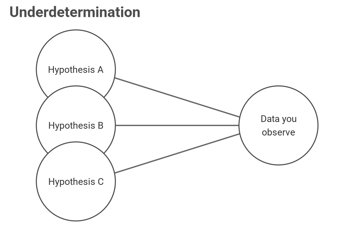
Many competing, mutually exclusive hypotheses could explain the observed data. The data contains patterns and associations to help you test an already established causal model, but the data alone is silent on what the right data-generating process is. That process is what you're trying to encode with a causal and statistical model. Moreover, when forecasting, historical data may be unavailable. It is the subject-matter expert who can design the causal model. The one who understands the "physics," the context, of what must happen between reality and your observed data. This knowledge is the actuary's value proposition: "I'm the expert in how insured event [X] is claimed, adjudicated, paid, and ultimately gets recorded in the data you query to forecast future frequency and severity of [X] so it can be priced for future underwriting and all done within government regulation and standards of practice." The causal model is the priority, and the statistical one is less so.
You can have the same data and the same statistical methods, yet propose two different causal models that lead to different conclusions. The causal model implies different realities or different queries. The query or forecast goal, the causal model, and the statistical model should all align. Failing to have a clear causal model invites trouble.
Not a Paradox
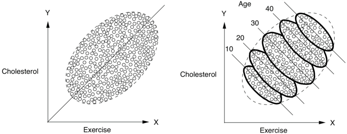
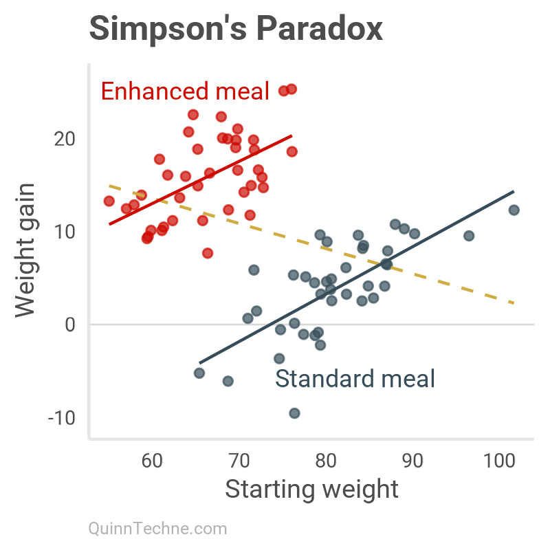
Here is a special case of trouble. Using the same data and model tool, but with different causal models, can lead to Simpson's paradox. The so-called paradox is the confusion of seeing strong correlations within subgroups, but when those subgroups are aggregated, the correlation disappears or even reverses!
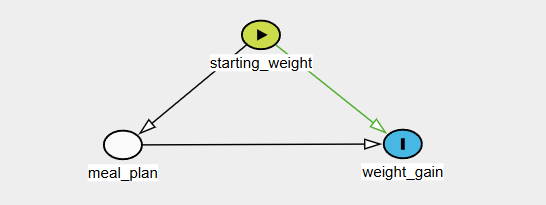
But it's no paradox, it's the consequence of unspecified causal models. Let's do our own example. Suppose you're interested in students' weights over a semester, noting there are two meal plan options (standard or enhanced):
The query: How does starting weight directly affect weight gain?
- Initial starting student weights, starting_weight
- Binary cafeteria meal plan, meal_plan
- Weight gain during the semester, weight_gain
set.seed(20260430)
n <- 80

alpha_true        <- 0.0     # Baseline weight gain
beta_starting     <- 0.50    # Heavier gain more
beta_meal_plan    <- 20.0    # Enhanced-meal boost
sigma_assign      <- 5.0     # Treatment assignment noise
sigma_resid       <- 3.5     # Observational noise

starting_weight <- rnorm(n, mean = 75, sd = 10)

# Meal plan assignment depends on weight (0 = standard, 1 = enhanced)
meal_plan       <- as.integer(starting_weight + rnorm(n, 0, sigma_assign) < 75)

weight_gain     <- alpha_true +
                   beta_starting  * (starting_weight - 75) +
                   beta_meal_plan * meal_plan +
                   rnorm(n, 0, sigma_resid)
Causal Model No. 1:
Thinking that only the starting weight matters and meal plan has no bearing on weight gain.
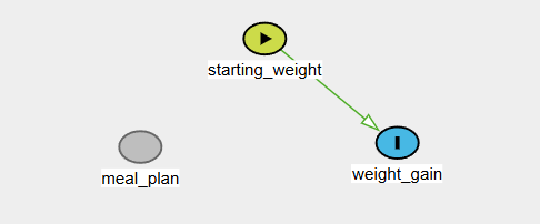
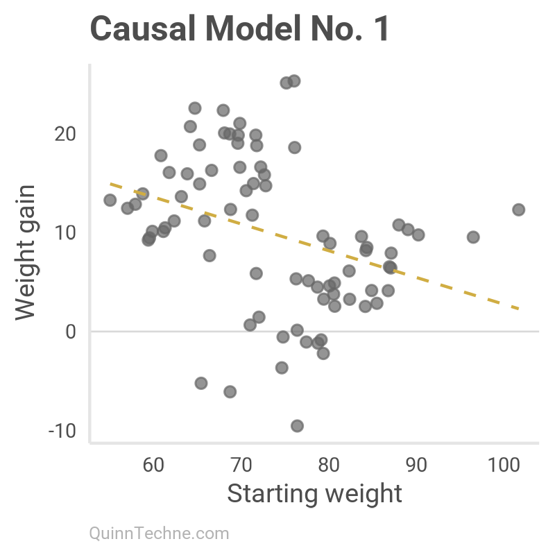
No arrows come or go from meal plan. The model is only interested in starting weight and weight gain, plotted and modeled here:
Call:
lm(formula = weight_gain ~ starting_weight, data = dat)

Residuals:
     Min       1Q   Median       3Q      Max
-18.6707  -4.1918   0.2104   4.6520  16.0707

Coefficients:
                Estimate Std. Error t value Pr(>|t|)
(Intercept)     29.80492    6.25257   4.767 8.52e-06 ***
starting_weight -0.27056    0.08407  -3.218  0.00188 **
Causal Model No. 2:
The meal plan was a non-random selection depending on the student's initial weight.
We will include meal_plan in the Causal Model 2 regression model, not because we care about its coefficient value, but because the DAG tells us it's a mediator and must be controlled for to estimate the direct effect of starting weight on weight gain.
Call:
lm(formula = weight_gain ~ starting_weight + meal_plan, data = dat)

Residuals:
     Min       1Q   Median       3Q      Max
-11.0675  -2.8265   0.2342   2.6475   7.4712

Coefficients:
                 Estimate Std. Error t value Pr(>|t|)
(Intercept)     -35.79121    5.29653  -6.757 2.38e-09 ***
starting_weight   0.48847    0.06492   7.525 8.33e-11 ***
meal_plan        19.25331    1.25520  15.339  < 2e-16 ***
The paradox emerges. Within each meal plan, the slope is positive (solid lines); aggregated, the slope flips negative (dashed line). You can see this sign flip in the negative coefficient for Causal Model 1 versus the positive coefficient for Causal Model 2.
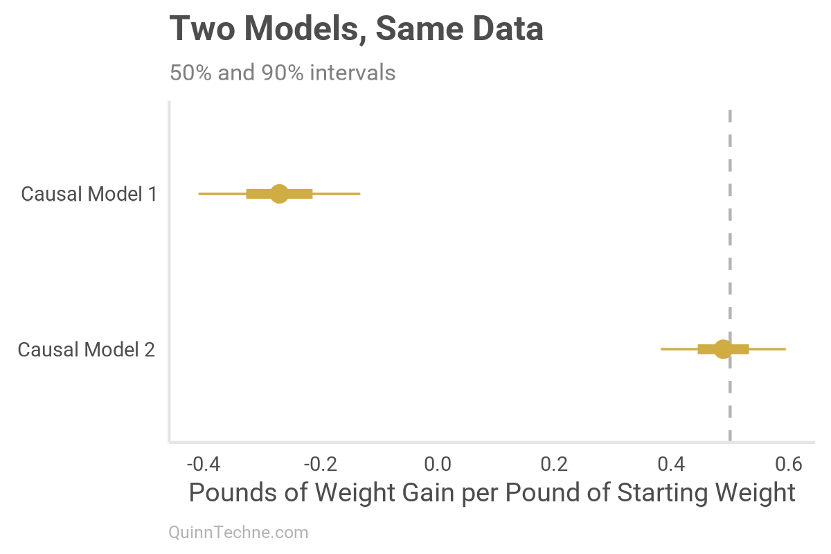
Causal Model No. 2 better reflects the data-generating process and recovers the effect (vertical dashed line). We can find it because we generated the data. But we are not so lucky as to know whether the model is sufficiently accurate when working with real-world data.
It’s Dangerous to Go Alone!
When modeling, ensure you have a causal model. Even better, make it explicit, write it down, and vet it. Doing this early in a project will help align your goal and statistical model. In out-of-sample, out-of-distribution cases, a causal model is all you get. Unfortunately, even if all these steps are done correctly, there is no assurance that it is the right model. Competing causal models can be empirically indistinguishable. Yet still, state your model. Justify it. Think of what it precludes and test those preclusions. By having a causal model, you will be less likely to wander from The Way and into biased, incoherent, or confusing outcomes.
McElreath, R. (2023). Statistical Rethinking (2023 Edition) [Computer software]. GitHub. https://github.com/rmcelreath/stat_rethinking_2023
Pearl, J., & Mackenzie, D. (2018). The Book of Why: The New Science of Cause and Effect. Basic Books.
Textor, J. (n.d.). DAGitty — Draw and Analyze Causal Diagrams [Computer software]. Retrieved April 26, 2026, from https://dagitty.net/
Calculations and graphics done in R version 4.3.3, with these packages:
Wickham H, et al. (2019). Welcome to the tidyverse. Journal of Open Source Software, 4 (43), 1686. https://doi.org/10.21105/joss.01686
Wilke C, Wiernik B (2022). ggtext: Improved Text Rendering Support for 'ggplot2'. R package version 0.1.2. https://CRAN.R-project.org/package=ggtext
The views and opinions expressed in this article are those of the author and do not represent the official policy or position of any employer, organization, or entity. This article is for informational and educational purposes only and does not constitute professional actuarial advice.
Generative AIs like Anthropic's Claude Opus 4.7 were used in parts of coding and reviewing the writing. ChatGPT generated the cover art.
