
When data visualization is not an option.
Excuse Me, Waiter
Tables are nice grids that hold numbers, text, or both together, hopefully transferring insights to the reader in a way that prose or visualizations cannot. They hold values, and the reader compares them across rows or columns, sometimes combining parts mathematically to calculate totals—this value, plus that, multiplied by that factor, and ta-da! The table's author may also wish to convey volatility in the table, perhaps by showing point-estimate means with associated standard deviations or by presenting a smorgasbord of scenarios across the table.
This is where it gets tricky: What if I want the table to show volatility for all the parts? For example, A + B = C, and show volatility for each of the three?
There are tradeoffs.
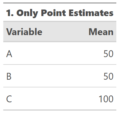
Method No. 1: Only Point Estimates
Back to A + B = C. Underlying these estimates are distributions with these normal (bell-shaped) distributions, where B varies more than A:
sim_data <- tibble(
  A = rnorm(n = 1e5, mean = 50, sd = 5),
  B = rnorm(n = 1e5, mean = 50, sd = 15),
  C = A + B
)
And plotted:
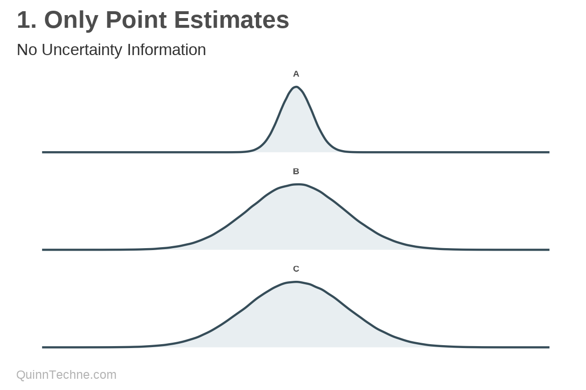
You could ignore the fact that these are probabilistic distributions and show only means. But where's the fun in denying your audience context? If you are estimating an amount, it has a probability distribution.
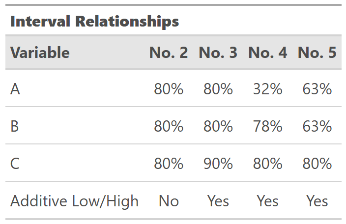
Method No. 2: Independent Intervals
You could show intervals, the range of values that capture a percentage of the distribution. Higher volatility is a wider range, and lower volatility a smaller range all for the same percentage of the distribution. The dotted blue lines represent an 80% interval, calculated independently within A, B, and C.
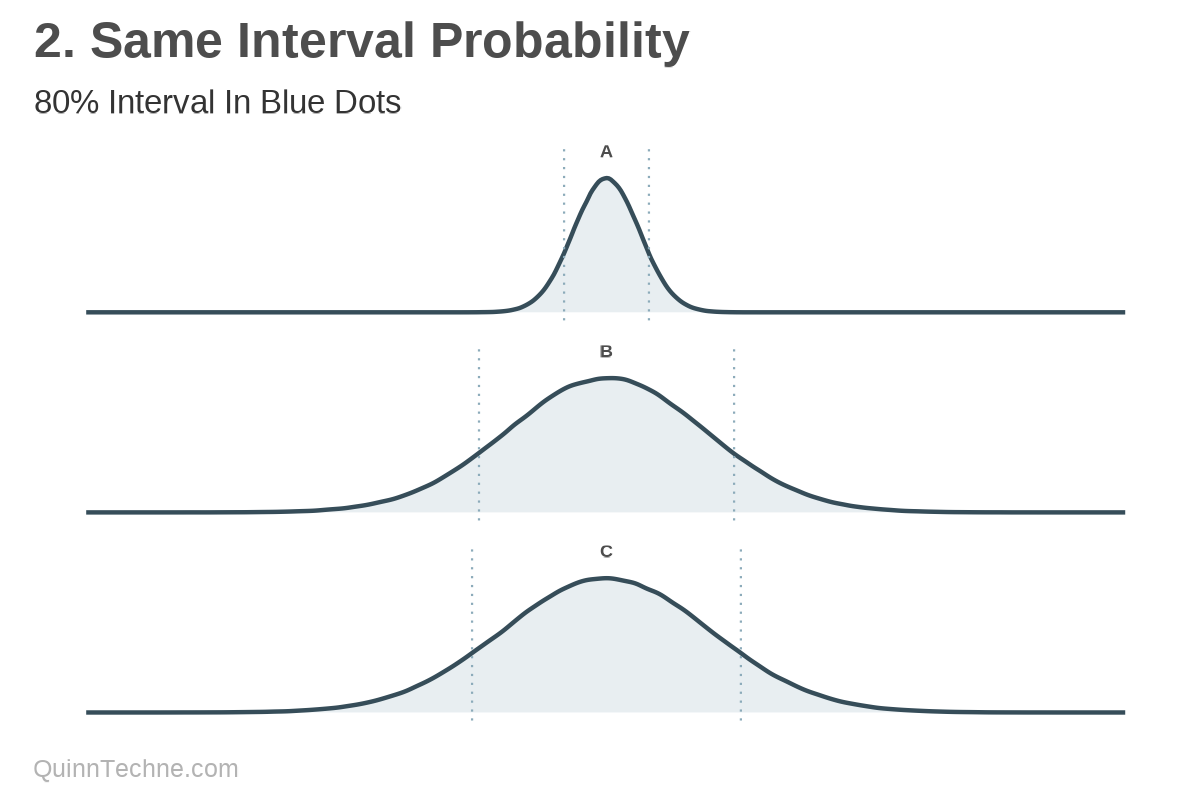
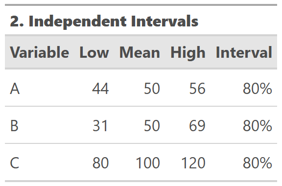
But it starts breaking down: A + B = C doesn't hold for the low and high bounds of the intervals. It's jarring to the audience if they expect A + B = C, and the table doesn't make that immediately obvious.
Method No. 3: Additive Constraint
The goal is then to convey volatility while preserving an expected relationship between A, B, and C. What if you calculate A and B, and then add their results?
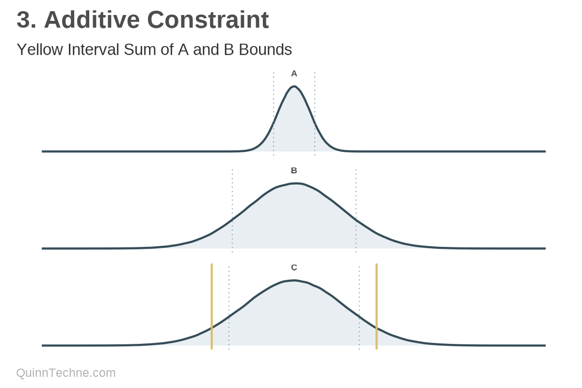
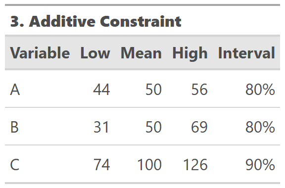
Unfortunately, percentile values, the low-high bounds, are not additive. Instead, C is exaggerated beyond the 80% intervals of its parts, which is also marked in the yellow solid lines in the chart.
Method No. 4: Conditional Sampling
One could calculate the 80% interval of C and then find the average values of A and B given a filtering around C's 80% percentile values.
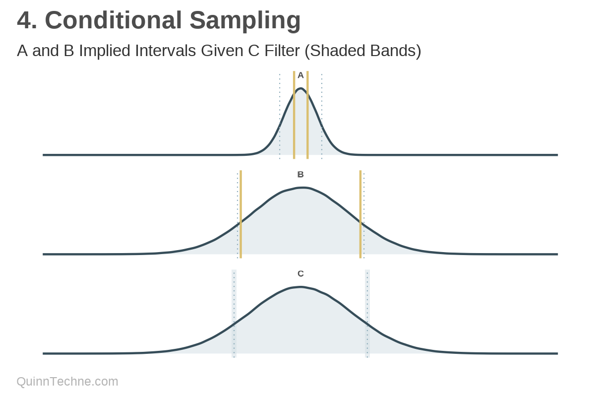
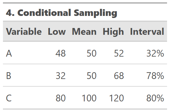
Now the parts are adding up as expected. However, the back-calculated intervals of parts A and B vary. Remember, B is the higher variance parameter, and see how it drives C's result.
Method No. 5: Perfect Correlation
A variation on Method No. 4 is to find C's interval first, and then work backwards for what A and B get you that value while constraining A and B to have the same interval.
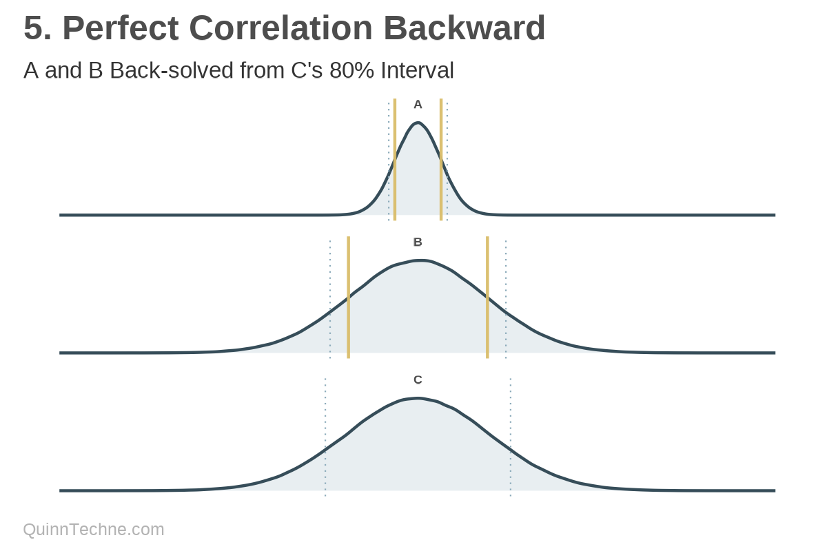
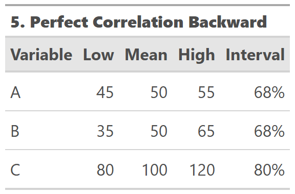
This method forces A and B to be perfectly correlated. The intervals are a function of each distribution's standard deviation. Recall that A has a standard deviation of 5 and B has 15. They must move in this ratio to maintain the same interval. As we learned in Method No. 2, interval values are not additive; thus, to sum to C's 80% interval, A and B compress to smaller intervals than that. However, forcing correlation where none might be seems dangerous.
Other Cases
From the prior code chunk, we can see that A and B are independent distributions. As the correlation between A and B becomes stronger, some of these methods produce intervals with less contrast, closer to C's interval, because A and B are moving in sync.
We can also see that A and B are additive and normally distributed. These methods hold with skew, but I did not test them for multimodal distributions (they have their own challenges with intervals in general). Multiplicative A and B intervals can be calculated in similar ways. However, as soon as you move beyond independent, additive, and normal distributions, I recommend using simulations to help with these types of calculations. Which, I'll put in my plug for Bayesian methods, because all the complexity of joint probability distributions and the uncertainty of the parts are automatically captured in the posterior distributions.
But for tables, unfortunately, no method consistently yields consistency in all parts.
Visualizing these intervals is easier than communicating them in tables. If you only have a table, keep all the intervals the same and note that the interval values won't follow the same mathematical rules as the means.
For a table involving discrete scenarios, consider Method No. 4 as a starting point, as A and B can be further adjusted to "tell the story" of the scenario. It would be beneficial to communicate the likelihood of the scenario based on the inputs provided. The final scenario value may seem common, but if the inputs are unlikely values, then the entire scenario is unlikely. Method No. 4 tries to maximize what input values you might see given the outcome (C, in this case).
Sometimes the tool, model, or number of displayed parts limits your ability to display all the intervals. In this case, demonstrate how to build up the final result using point estimates and then display intervals on the final results. However, this means you need to provide context for what drives that final interval. Context is key.
Calculations and graphics done in R version 4.3.3, with these packages:
Iannone R, et al. (2024). gt: Easily Create Presentation-Ready Display Tables. R package version 0.11.0. https://CRAN.R-project.org/package=gt
Qiu Y (2024). showtext: Using Fonts More Easily in R Graphs. R package version 0.9-7. https://CRAN.R-project.org/package=showtext
Wickham H, et al. (2019). Welcome to the tidyverse. Journal of Open Source Software, 4 (43), 1686. https://doi.org/10.21105/joss.01686
Generative AIs like ChatGPT, and Claude were used in parts of coding and writing. The cover art was created by the author using Midjourney and GIMP.
This website reflects the author's personal exploration of ideas and methods. The views expressed are solely their own and may not represent the policies or practices of any affiliated organizations, employers, or clients. Different perspectives, goals, or constraints within teams or organizations can lead to varying appropriate methods. The information provided is for general informational purposes only and should not be construed as legal, actuarial, or professional advice.
