
The point of this example is not to praise R² but to bury it. —Richard McElreath, Statistical Rethinking
Models' Waistlines
Perhaps it's the trauma of a STAT 101 course that instills in many the use of R² (R-squared, or Coefficient of Determination if you want to be bougie about it) as a measure of a regression model fit for making predictions. But it's a bad measure. We can do better.
$$R^2 = 1 - \frac{SS_{\text{residual}}}{SS_{\text{total}}} = 1 - \frac{\sum_{i=1}^{n}(y_i - \hat{y}_i)^2} {\sum_{i=1}^{n}(y_i - \bar{y})^2}$$
\( y_i \), observed values
\( \hat{y}_i \), predicted values
\( \bar{y} \), mean of observed values
\( SS_{\text{residual}} \), residual sum of squares
\( SS_{\text{total}} \), total sum of squares
As a reminder, for simple regression models, R² is a ratio of the variance explained by the variable being predicted. It's desirable to have it closer to a value of 1.0, as this indicates that your line is fitting to the data closely.
But here's the kicker.
R² increases monotonically with the addition of every model parameter. Thought \(x_1\) predict \(y\) well? Then you'll love \(y\) predicted by \(x_1\) through \(x_5\)!
Suppose you have increasingly complex models: Parameters 1 and 2 are signals—the true model, but 3, 4, and 5 are noise.
# Where x1–x5 are draws from a standard normal distribution
y <- 0 + 0.15 * x1 - 0.40 * x2 + rnorm(n_obs, 0, 0.5)
$$y = \beta_1 x_1$$
$$\mathbf{y = \beta_1 x_1 + \beta_2 x_2}$$
$$y = \beta_1 x_1 + \beta_2 x_2 + \beta_3 x_3$$
$$y = \beta_1 x_1 + \beta_2 x_2 + \beta_3 x_3 + \beta_4 x_4$$
$$y = \beta_1 x_1 + \beta_2 x_2 + \beta_3 x_3 + \beta_4 x_4 + \beta_5 x_5$$
Notice the direction of R² in this table as we fit additional parameters.
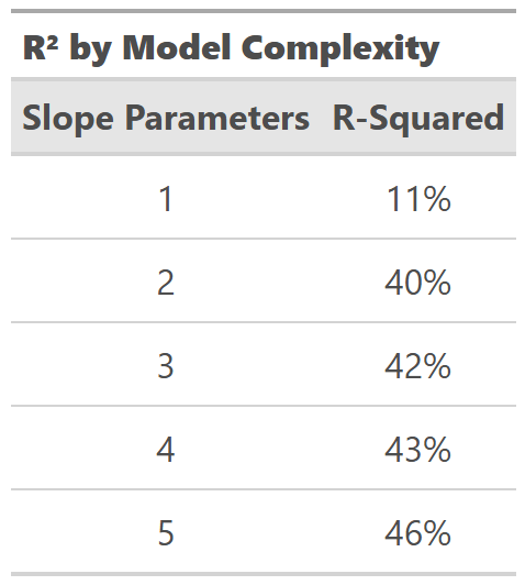
The value of R² increases monotonically with every new parameter—signal or noise.
To paraphrase Richard McElreath: linear regression is unreasonably effective. However, it tends to overfit the data even with a few parameters because it's trying to optimize shrinking the squared differences between data and the line, making the model exictiable by outliers. Overfitting is the default behavior of linear regression.
In-N-Out Fitters
To illustrate, we will use the same five-slope model from before, but this time we will use cross-validation to look at fits in and out of sample. First, we randomly split the data into in-sample training and out-of-sample testing 50%/50% (n = 30 each). The in-sample fit is measured on the same data the model was trained on. However, the out-of-sample fit will be measured on the remaining data that the model was not trained on. Here is the R² result:
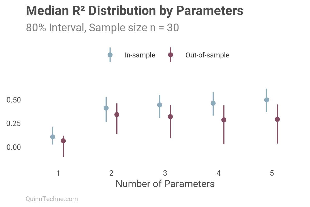
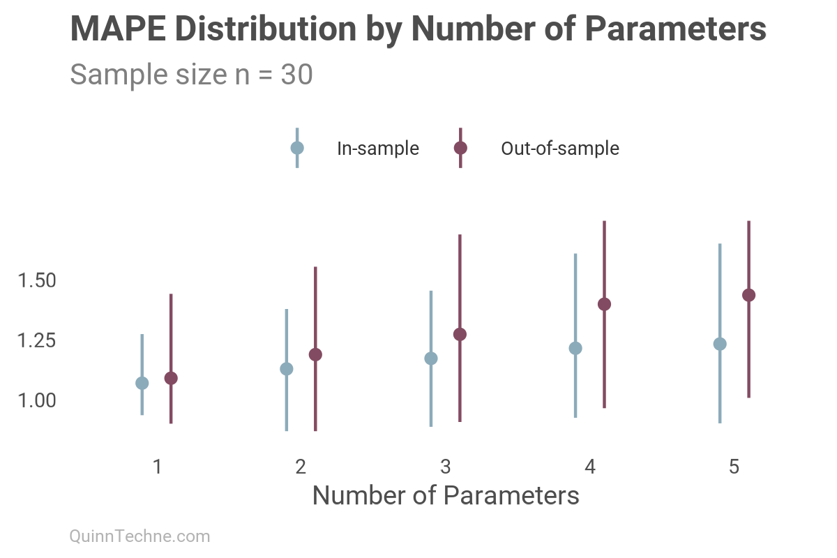
Note how the model always shows a better in-sample fit, closer to 1.0 with each added parameter. We can see similar in-out behavior in other deterministic model fit measures, like Mean Absolute Error (MAE) or Mean Absolute Percentage Error (MAPE), where a value closer to zero is desirable:
Unlike R², MAPE will not always increase with added parameters. This alone would make MAE or MAPE a better default fit measure than R². However, you can see the out-of-sample fit worsen (higher values) at a faster rate than in-sample would show. Again, the fit we should be interested in is the out-of-sample fit.
Wild Fits
I'm dismayed at how pervasive R² is still used among actuaries. Here is a recent example. An actuary wrote a trade journal piece about possible ways to improve federal risk-adjustment models. These models predict the relative morbidity of enrollees, which affects how much health insurance companies are paid. Moreover, these models move a lot of money around, so it's commendable to take the time to explore their improvement. Unfortunately, the author's design choices in model fit statistics muddy the insights.
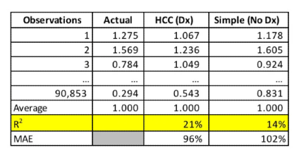
This table aims to compare two models, where "HCC (Dx)" has more variables, maybe 100 more, than "Simple (No Dx)". Of all the options, the author literally highlights R². However, our knowledge of the ever-increasing R² confounds attempts to assess whether one model is a better predictor than the other. The 21% versus 14% difference doesn’t alone establish superior predictive ability:
Of course, the model with more parameters has a higher R²!
I emailed the author and suggested showing out-of-sample distributions of R² or MAE to enhance this table.
Out-of-sample Without The Work
Ah, but what if I cannot be bothered with all the loops and simulations to get out-of-sample fits? For starters, many nice packages will do it for you. Two, generative AI can write you all the loops and simulations. But third, there are model fit statistics designed to approximate the out-of-sample fit. These are information criteria measures. Here's a common one:
$$\text{Akaike Information Criterion (AIC)} = -2 \log(L) + 2k$$
\( L \), maximum likelihood of the fitted model
\( k \), number of parameters in the model
For small sample sizes, there's AICc (small-sample corrected). For Bayesian models, you also have options like Deviance Information Criterion (DIC) and Watanabe-Akaike Information Criterion (Widely Applicable Information Criterion, or WAIC).
Unlike deterministic measures like R² or MAPE, these measures are probabilistic and penalize complexity according to the expected degradation in predictive performance.
To illustrate, here is the same simulation as prior charts, showing both the out-of-sample deviance \(-2 \log(L)\), which measures how well the model encodes the data, and the in-sample AIC measure, where lower values indicate better fit.
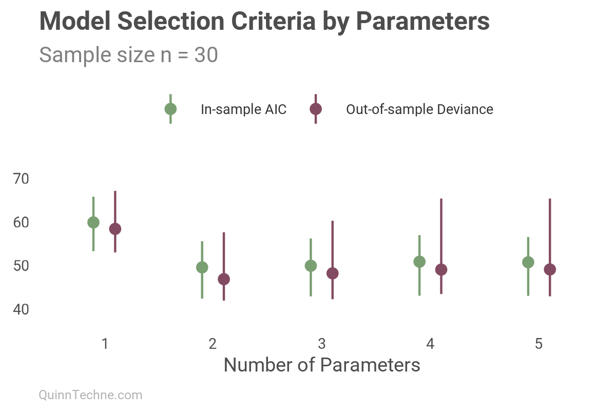
Notice how AIC (green), even though in-sample, tracks well with the out-of-sample deviance. Their similarity across parameter counts is what makes it a good fit statistic. This approximation of out-of-sample, and out-of-sample metrics in general, are a better choice for comparing predictive models than in-sample metrics prone to overfitting.
Here's an AIC calculation in the programming language R to understand what goes into \( L \):
# Sample data and linear regression
y <- c(3, 4, 5, 6, 8)
x <- c(1, 2, 3, 4, 5)
fit <- lm(y ~ 1 + x)
# Calculate from first principles
y_hat <- fitted(fit)
residuals <- resid(fit)
n <- length(y)
sigma_hat <- sqrt(sum(residuals^2) / n)
# Likelihood assuming normal errors
L <- prod(dnorm(y, mean = y_hat, sd = sigma_hat))
log(L)
[1] -0.7803711
# Log-likelihood explicitly log(a × b) = log(a) + log(b)
log_L <- sum(dnorm(y, mean = y_hat, sd = sigma_hat, log = TRUE))
[1] -0.7803711
# Extract log-likelihood directly from lm()
logLik(fit) # built-in function
-0.7803711 (df=3)
# AIC Calculation
-2 * log_L + 2 * 3 # k = 3: intercept, slope, sigma
[1] 7.560742
AIC(fit) # built-in function
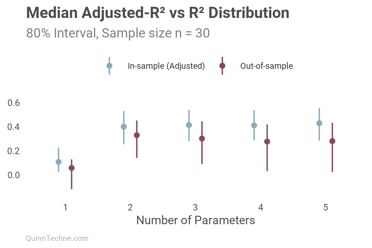
[1] 7.560742Hey, but isn't there an Adjusted-R² that penalizes additional parameters like AIC?
$$R^2_{\text{Adjusted}} = 1 - \frac{(1 - R^2)(n - 1)}{n - p - 1}$$
\( R^2 \), from before
\( n\), number of observations
\( p \), number of predictors
As shown, there is an adjusted version of R², which has the right idea to penalize complexity, but the penalty isn't based on information criterion like AIC. As a consequence, we still see overfitting in-sample with a slight continual rise, while the out-of-sample deteriorates downwards. It's better than vanilla R², but not by much.
Design Choices
- Some fit metrics are interpretable while others are not. For example, if using MAPE, you can say your observations will be ±X% from the forecast on average. Whereas, AIC, the number has no meaning other than relative to other AIC fits on the same data.
- Out-of-sample measures are more likely to generalize to future forecasts than in-sample measures, which tend to be overly optimistic. In-sample results can be useful for a quick gut check, but consider the value of reporting out-of-sample distributions of model fits, as this provides better context for your audience.
- Most information criterion statistics approximate the out-of-sample fit while being calculated in-sample.
One has many model fit statistics to choose from. You can always do better than in-sample R².
McElreath, R. (2020). Statistical Rethinking: A Bayesian Course with Examples in R and Stan (2nd edition). Chapman and Hall/CRC. https://xcelab.net/rm/. See Chapter 7 "Ulysses' Compass" for related details.
Mehmud, S. M. (2025). Simplifying Risk Adjustment. Society of Actuaries. https://www.soa.org/sections/health/health-newsletter/2025/may/hw-2025-05-mehmud/
Wikipedia contributors. (2025). Coefficient of determination: Adjusted R². Wikipedia. https://en.wikipedia.org/wiki/Coefficient_of_determination#Adjusted_R2
Calculations and graphics done in R version 4.3.3, with these packages:
Iannone R, et al. (2024). gt: Easily Create Presentation-Ready Display Tables. R package version 0.11.0. https://CRAN.R-project.org/package=gt
Qiu Y (2024). showtext: Using Fonts More Easily in R Graphs. R package version 0.9-7. https://CRAN.R-project.org/package=showtext
Wickham H, et al. (2019). Welcome to the tidyverse. Journal of Open Source Software, 4 (43), 1686. https://doi.org/10.21105/joss.01686
Generative AIs like ChatGPT, and Claude were used in parts of coding and writing. The cover art was created by the author using Midjourney.
This website reflects the author's personal exploration of ideas and methods. The views expressed are solely their own and may not represent the policies or practices of any affiliated organizations, employers, or clients. Different perspectives, goals, or constraints within teams or organizations can lead to varying appropriate methods. The information provided is for general informational purposes only and should not be construed as legal, actuarial, or professional advice.


