
An assumption ignored is still an assumption made.
Feeling the Confusion
I've seen three kinds of timid statistical modeling behaviors:
- Giving up on modeling an assumption when faced with uncertainty.
- Adding implicit conservatism when uncertain.
- Uncertain about a data-driven forecast and adjusting it back to expectations.
These issues arise from failing to think in explicit statistical distributions. Distributions are all possible values of something and how plausible they are. Most distributions are described with a center (like mean, median) and spread (like standard deviation, variance), among other statistics. Spread is where the risk is. Actuaries are portrayed as risk experts, yet I see many models that only track the center, no spread—no measure of risk.
Encoding Uncertainty
By building a model, we externalize our hypotheses and assumptions about a phenomenon's causes and effects. The model converts our background information and data into something checkable, the cornerstone of science.
This externalization and explicitness are important because it is much harder to critique what is absent. Omitted assumptions are hard to recall. It is like reverse availability bias: recalling a recently seen model assumption is easy, but contrast that with the chances of remembering to recall background information important to the model that's absent, and there's no clue in the model to trigger that memory.
One modeling input to make explicit is uncertainty. Uncertainty is a function of your knowledge, not reality. We have incomplete background information, noisy data, and future contingent events. The modeler will always be faced with uncertainty.
If the uncertainty seems overwhelming, that's no excuse for inaction. Distribution spread is where that uncertainty is encoded—no matter how big or small, distributions can handle it.
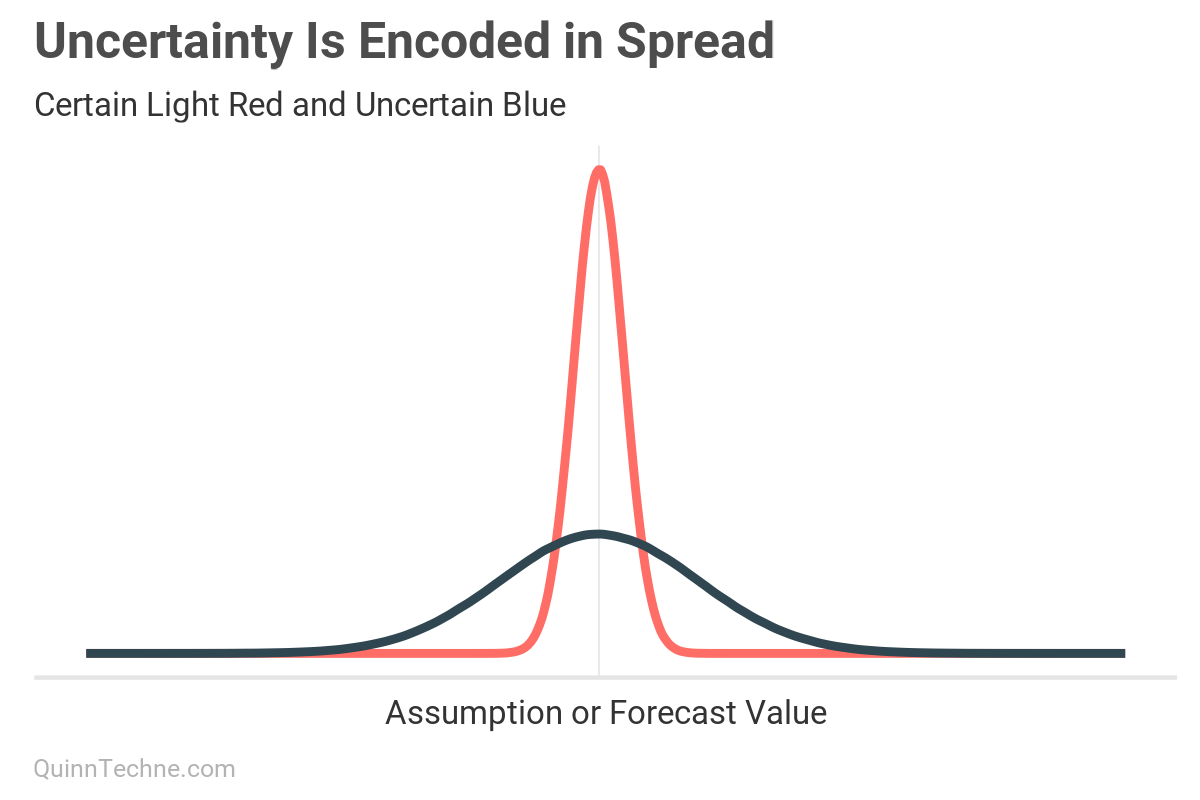
Here, the blue distribution is less certain, with a larger standard deviation. The blue distribution covers more plausible values with its wider spread. The light red distribution is more certain and shows fewer plausible values under its curve because it has a lower standard deviation. It is more certain where the value is.
High uncertainty is no reason to abandon modeling. Suppose there is a highly uncertain assumption that could add or subtract from a forecast. Because adding zero, no adjustment, is a plausible value, the modeler foregoes an explicit adjustment. However, by skipping encoding that uncertainty, the final forecast will be missing that source of uncertainty. Having well-quantified uncertainty can be valuable context.
For example, consider Actuarial Standards of Practice (ASOP) No. 56 — Modeling:
"Items the actuary should consider...the model's ability to identify possible volatility of output, such as volatility around expected values."
Knowing the spread around expected values can also help with ASOP No. 41 — Actuarial Communications:
"The actuary should consider what cautions regarding possible uncertainty or risk in any results should be included in the actuarial report."
By thinking in distributions, the modeler can encode the uncertainty and propagate it to the final forecast while having explicit and checkable modeling.
Hiding Conservatism
Uncertainty can be encoded in a distribution's spread. Yet, I see modelers skip this step and go straight to conservatism. It is okay to have conservatism, and regulation sometimes requires it. It's okay if uncertainty is the motivation to add conservatism. But hopefully, it crosses the modeler's mind that uncertainty is also encoded as spread. Here's why.
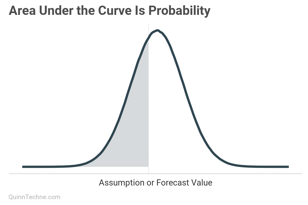
The area under a distribution curve is a probability. Here, the blue shaded area is the probability of a value equal to the gray vertical line or smaller.
Conservatism is a different probability outcome than uncertainty: uncertainty changes the spread whereas conservatism shifts the center.
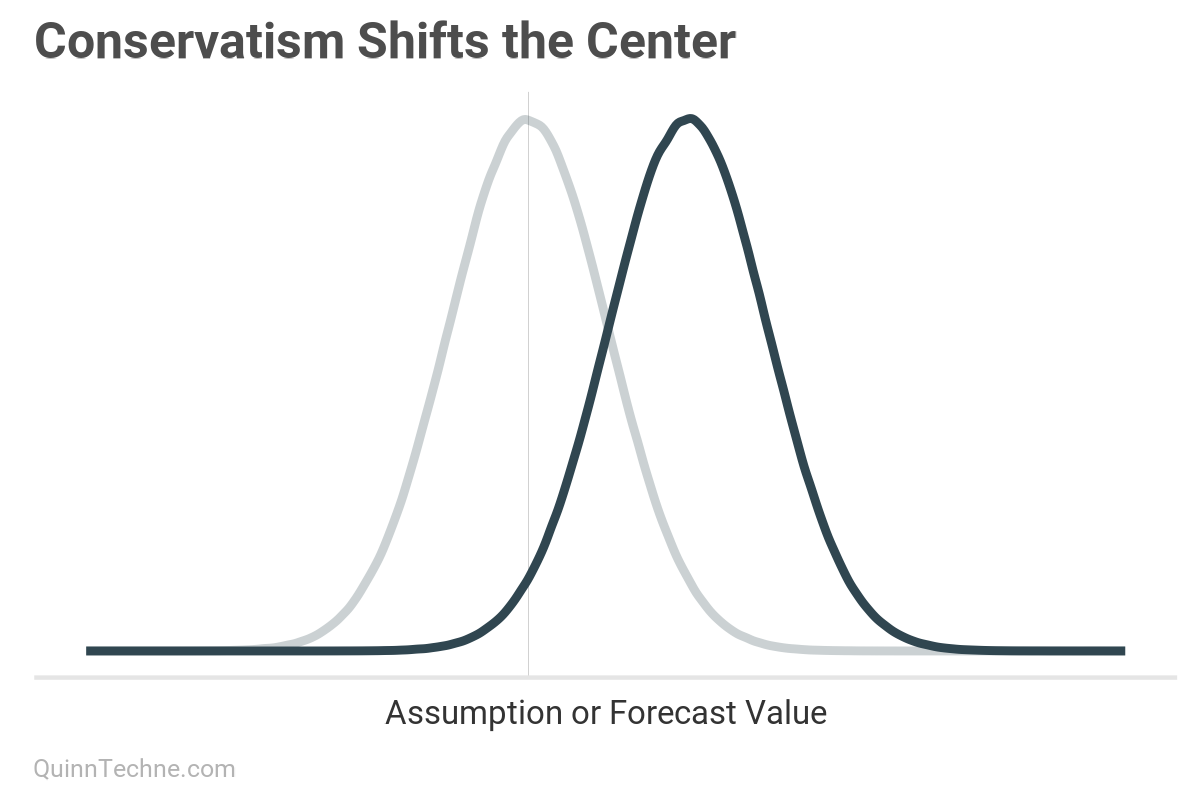
The "I'm uncertain; thus, I will be conservative" conflates uncertainty, spread, and conservatism by skipping spread. For example, when conservatism is added, the blue distribution is shifted to the right. But from before, spread changes the shape, not the location of the distribution. If the encoding-uncertainty-as-spread is skipped, the modeler has no way of knowing how they changed the probability of the outcome.
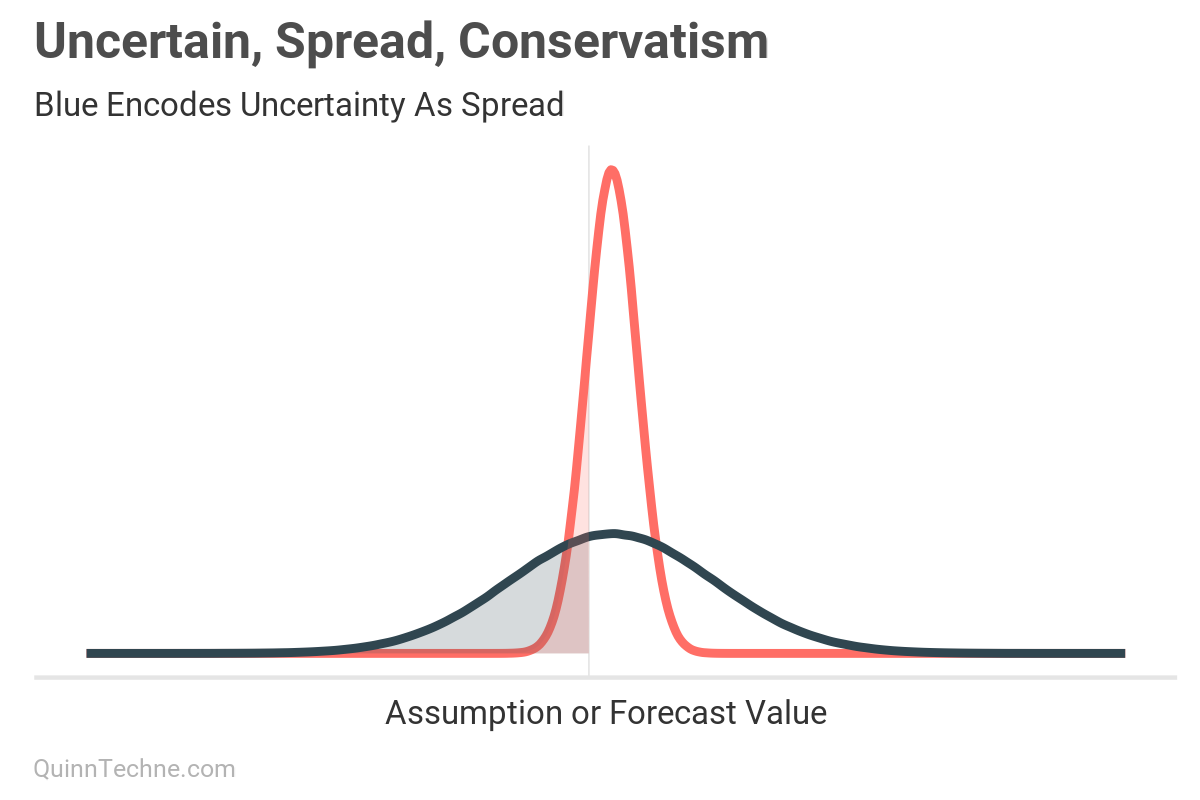
Notice the different sizes of the shaded areas. Suppose the shaded area is the possibility of a loss. The red area is smaller than the wider blue area because the blue area encodes uncertainty as spread, in addition to being shifted by conservatism. If conservatism is added because of uncertainty but the spread is not updated to encode that uncertainty, you get an overconfident light red distribution shown as the smaller red area, understating the risk of a loss.
Layering in conservatism here and there is alluring because there usually is an asymmetrical incentive in under versus over-forecasting a value. One might think it's better to tell the boss it will cost X when it's more plausible it will cost less than X.
The modeler has biased the forecast by introducing conservatism. It is now systematically different from trying to forecast accurately with the given information. This layering is dangerous when implicit conservatism occurs—when conservatism is smuggled into other assumptions. If the conservatism is implicit, the modeler has lost track of how much bias there is while conflating other assumptions with it. They're flying blind.
This conservatism bias is pervasive enough that it has been directly addressed in otherwise broad principle-based guidance: ASOP No. 56 — Modeling:
"While assumptions might appear to be reasonable individually, conservativism or optimism in multiple assumptions may result in unreasonable output."
When modeling, seek first to forecast as accurately as possible, given the available background information, model, and data at the time. First, uncertainty is encoded as spread. Then, later, add explicit conservatism if justified.
Noisy Data, Noisy Brains
I have been in discussions where the model forecast is noticeably different than stakeholders' prior expectations. I will describe the model, assumptions, and data, but sometimes this fails to persuade, and the conversation terminates with someone declaring, "Well, you can never know what will happen."
True.
Which is why we need models.
We don't model probabilistically because we believe in perfect forecasts; we model because it beats chaos. When someone claims to rely on "years of experience" or "actuarial judgment" without a model, they're still using a model—just one that's invisible, prone to inconsistency, and uncheckable unless externalized. We want models that are adequate for making decisions under uncertainty, can explain past observations, and forecast future ones.
Another outcome I see when forecasts disagree with prior expectations is to tinker with the outcome until it aligns with prior expectations. There are two risks here:
- It may be a wasted effort. If the model tracks spread, the prior expectation may very well be a plausible value within the forecast's distribution. No further action is required. However, no formal inference can occur if the model forecast lacks spread.
- Tinkering with the forecast can be a path to confirmation bias. Here's an excerpt from an American Academy of Actuaries 2023 issue brief:
"The actuary does not see the results they expect, so they continue to tweak the model until they eventually arrive at a scenario that confirms their existing bias. The actuary will then likely favor this outcome. By becoming aware of confirmation bias, actuaries can be more open to accepting results that do not confirm their original hypotheses."
Now, a better next step when seeing unexpected forecasts is to review the model's assumptions, data, and structure. Maybe seeing the forecast triggers a new insight into the causal model or generates a new hypothesis yet thought of. A closer inspection of the data could show it was sampled differently than first thought. Or the causal model could be better mapped to model parameters, including changing the number of parameters while checking out-of-sample model-fit diagnostics and remaining faithful to background information.
This advice is also found in general forecasting practices, like Forecasting: Principles and Practice (and note another conservatism bias warning!):
"We should only adjust when we have important extra information which is not incorporated in the statistical model. Hence, adjustments seem to be most accurate when they are large in size. Small adjustments (especially in the positive direction promoting the illusion of optimism) have been found to hinder accuracy, and should be avoided."
New data or thoughtful reparameterization could make the forecast more certain, but it will never eliminate uncertainty. Understand the advantages and limitations of your background information, data, and models.
Confidence in Uncertainty
As a parting note, models are a simplification of reality. One common unstated assumption is that the forecasted future will mostly look like the status quo: no nuclear winter, societal collapse, or AI singularity (yet...). Your background assumptions and model should focus on salient model parameters, where the uncertainty should be focused, too. If your model context includes fat-tailed risks, select distributions that properly encode the increased probability of outliers, making these assumptions as explicit and checkable as any other.
It's easier to hide behind ad-hoc complex models and industry jargon than to say: "Here's what we know and how we know it, and here's the range of possible forecasts given our current knowledge, model, and data." Be bold and encode your uncertainty.
American Academy of Actuaries. (2023, July). Risk Brief: Understanding Data Bias. https://www.actuary.org/sites/default/files/2023-07/risk_brief_data_bias.pdf
Actuarial Standards Board. (2009, December). Actuarial Standard of Practice No. 41 — Actuarial Communications. American Academy of Actuaries. https://www.actuarialstandardsboard.org/wp-content/uploads/2014/03/asop41_secondexposure.pdf
Actuarial Standards Board. (2019, December). Actuarial Standard of Practice No. 56 — Modeling. American Academy of Actuaries. https://www.actuarialstandardsboard.org/wp-content/uploads/2020/01/asop056_195-1.pdf
Jaynes, E. T. (2003). Probability Theory: The Logic of Science. Cambridge University Press. http://www.med.mcgill.ca/epidemiology/hanley/bios601/GaussianModel/JaynesProbabilityTheory.pdf
Hyndman, R.J. & Athanasopoulos, G. (2021). Forecasting: Principles and Practice, 3rd Edition. Otexts. https://otexts.com/fpp3/
McElreath, R. (2020). Statistical Rethinking: A Bayesian Course with Examples in R and Stan (2nd Edition). Chapman and Hall/CRC. https://xcelab.net/rm/
Calculations and graphics done in R version 4.3.3, with these packages:
Wickham H, et al. (2019). Welcome to the tidyverse. Journal of Open Source Software, 4 (43), 1686. https://doi.org/10.21105/joss.01686
Generative AIs like ChatGPT, Claude, and NotebookLM were used in parts of coding, and writing. Cover art was done by the author with Midjourney and GIMP.
This website reflects the author's personal exploration of ideas and methods. The views expressed are solely their own and may not represent the policies or practices of any affiliated organizations, employers, or clients. Different perspectives, goals, or constraints within teams or organizations can lead to varying appropriate methods. The information provided is for general informational purposes only and should not be construed as legal, actuarial, or professional advice.


