Rate Development Never Leaves the Distribution

Can't See the Joint Distribution for the Marginals

Nine Distributions Were Gifted to the Race of Men

A capitated rate is paid on a fixed, regular basis per member regardless of service use. The goal is to price it to pay for whatever associated costs it's meant to cover. Think of something akin to an insurance premium.

Rate development starts with historical data, then the actuary adjusts it to estimate future costs: changes in benefits, cost inflation, administrative costs, etc. It's forecasting.

Note how the rate is built from subcomponents, like a cost for benefits and non-benefit costs such as administrative expenses. Each one is a forecast, so each one has a distribution. For example, say we estimate total future administrative costs will be near \$45 per member per month (PMPM), though not exactly \$45. These values reflect what we consider plausible given our model, assumptions, and data at the time.

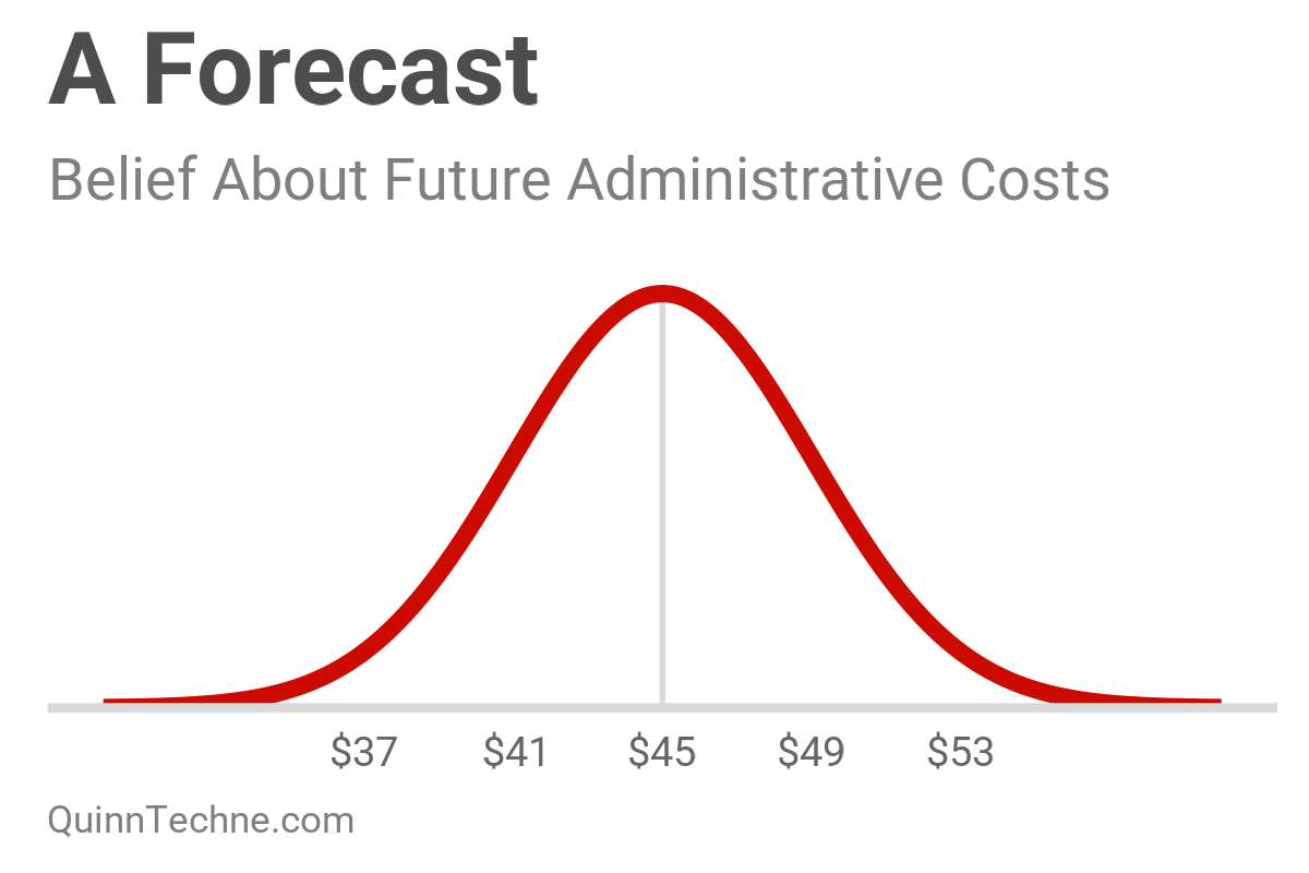
How do we then handle all these subcomponents as a holistic rate forecast?

The key is that all these rate components are part of one joint probability distribution. The mistake is treating them as individual pieces and forgetting how they combine as a whole.

A joint probability distribution is used when you predict more than one event, sometimes when the events are associated. For example, forecasting cold temperatures and the size of energy bills is a joint probability of two events, where a decrease in one is associated with increased values of the other. In Bayesian inference, the probability model is a joint distribution of anywhere from a few parameters to millions!

First, some forecasted components, across insurance types:

• Unpaid claims liability (some claims are still working their way through the system)
• Enrollment
• Known program, benefit, or law changes but an unknown financial impact
• Cost inflation trends, frequency trends
• Morbidity or selection drift; wear-off of underwriting selection
• Administrative costs

For each item, you have a random variable. A random variable is an unknown amount described by a distribution. In most cases, the random variable will one day be a realized value that you can score against what you predicted. Random variables will be denoted with a "~" tilde on top of them.

But some components are not random. We represent these variables as letters. They're somebody's choices. You don't have a distribution because there's no uncertainty to encode. You know the thing:

• Tax rates
• Assessment amount
• Risk margin

A special non-random variable is the decided capitation rate. Rate less costs is underwriting margin. The rate is a decision; the expected margin is computed; the realized margin is a random variable.

How Do You Turn This On?

Holistic handling begins with the random variables and their joint probability distribution. Here's an example with generic rating components:
$$\tilde{z} \sim p(\tilde{b}, \tilde{t}, \tilde{a} \mid y)$$

\( \tilde{z} \): The collection of all random rate components—the joint probability distribution.
\( \tilde{b} \): The financial impact of a known benefit change, in dollars PMPM.
\( \tilde{t} \): A prospective compound annual growth rate.
\( \tilde{a} \): A prospective administrative load.
\( y \): All probability is conditional probability. This \( y \) is shorthand for the model, assumptions adopted, all as of the information date. This conditional is my marriage of the Actuarial Standards of Practice ASOP No. 41, Actuarial Communications, the information date, and the Bayesian workflow of likelihood (model), priors (assumptions), and posterior update (data).
\( \sim \): "Is distributed as." The left side is a random variable; the right side is its distribution.
\( \mid \): The conditioning bar, read "given." The poster child of conditional probability.

It's in \( \tilde{z} \) that any covariance is also encoded. You may believe lower cost trends are associated with higher administrative loads. Well, you can encode that! Here's an example in R of a multivariate normal distribution (one way to do a joint probability distribution). You have a trend rate and an administrative load with a −0.5 correlation between them.

set.seed(42)

mu_z <- c(trend_rate = 0.05, admin_load = 1.10)
sd_z <- c(0.015, 0.02)
rho_z <- -0.5 # Lower trend goes with higher admin load

# Covariance = diag(sd) %*% correlation %*% diag(sd)
sigma_z <- diag(sd_z) %*% matrix(c(1, rho_z, rho_z, 1), 2, 2) %*% diag(sd_z)

n_draws <- 5e3
z <- MASS::mvrnorm(n_draws, mu = mu_z, Sigma = sigma_z)
head(z)
#    trend_rate admin_load
#[1,] 0.03421680 1.125794
#[2,] 0.04628719 1.083509
#[3,] 0.04284437 1.105123
#[4,] 0.04447596 1.112919
#[5,] 0.04889460 1.109644
#[6,] 0.05237939 1.098668

round(cor(z)[1, 2], 3)
# [1] -0.498 # Compare to rho_z

In notation, the model statement is:
 $$\tilde{z} \sim \text{MVN}(\mu, \Sigma)$$
$$\mu = \begin{bmatrix} \mu_1 \\ \mu_2 \end{bmatrix} = \begin{bmatrix} 0.05 \\ 1.10 \end{bmatrix}$$
$$\Sigma = \begin{bmatrix} \sigma_1^2 & \rho \sigma_1 \sigma_2 \\ \rho \sigma_1 \sigma_2 & \sigma_2^2 \end{bmatrix} = \begin{bmatrix}
0.000225 & -0.00015 \\ -0.00015 & 0.0004 \end{bmatrix}$$

\( \text{MVN} \): The multivariate normal distribution. It is a bell curve generalized to several variables at once.
\( \mu \): The vector of means, one per component.
\( \Sigma \): The covariance matrix—the spread of each component on the diagonal, and every pairwise covariance between them otherwise.

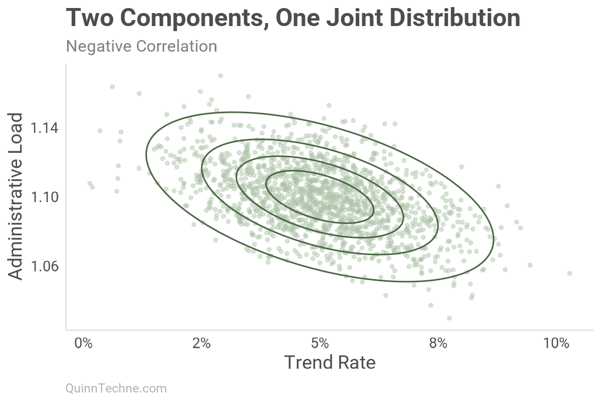
This chart shows the draws from our multivariate normal distribution. Note how higher trend draws pair with lower admin load draws. That's the negative correlation at work. You can extend this idea to any number of variables inside the distribution. It's a joint distribution that encodes your belief about capitation rate development.

The next step is to run the distribution through a cost-aggregating function. The function is context-specific. Here's a possibility:
  $$\tilde{c} = g(\tilde{z}) = (\text{known_paid} + \tilde{b}) \times (1 + \tilde{t})^{2} \times \tilde{a}$$

\( \tilde{c} \): The projected cost PMPM.
\( g(\cdot) \): The cost-aggregating function, the math that maps drawn samples into costs.
\( \text{known_paid} \): The incurred-and-paid base-period cost. We treat it here as a known number ($400 PMPM in our upcoming example).
\( 2 \): The known number of trend years between the midpoint of the base period and the rating period years.

Any equation that takes a random variable becomes a random variable itself even if other inputs are known, like the number of trend years or the known incurred and paid starting costs.

Next is to calculate a rate:
$$R = \frac{E(\tilde{c} \mid y)}{1 - m - x}$$

\( R \): The capitation rate. Note that it's not a random variable. It is a decision.
\( E(\cdot \mid y) \): The expectation operator or the probability-weighted mean over all outcomes, given the model, assumptions, and data at the time.
\( m \): The underwriting gain load. A chosen margin for solvency and financial needs (2% here).
\( x \): The premium tax rate (2.5% here).

Or, you could push the entire cost distribution through the loading instead, producing a distribution of indicated rates, where each one is the rate you would calculate if that cost draw were realized. You can use it to answer questions like, "What is the probability that a chosen \( R \) would deliver at least the underwriting load?"
$$\tilde{r} = \frac{\tilde{c}}{1 - m - x}, \qquad E(\tilde{r} \mid y) = R$$

\( \tilde{r} \): The indicated rate. This time it's random because \( \tilde{c} \) is.

The rate is a decision, but the uncertainty stays. It is now in the yet-realized underwriting margin given the rate.
$$\tilde{u} = \frac{R(1 - x) - \tilde{c}}{R}$$

\( \tilde{u} \): The realized underwriting margin as a percent of revenue.

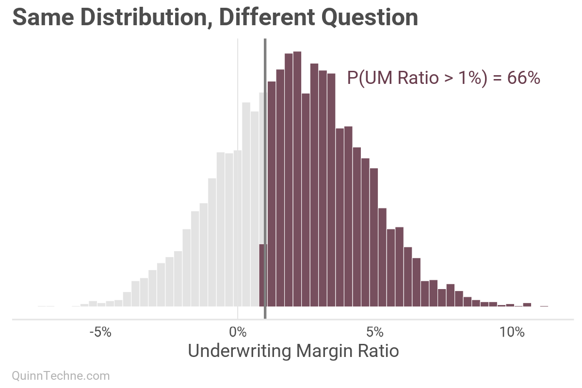
This is the predictive distribution of the underwriting margin: the distribution of a not-yet-observed quantity, calculated by inputting the components' joint predictive distribution through the aggregating cost function \( g(\tilde{z}) \). Its mean is the underwriting gain load. However, your belief about the underwriting margin is the whole distribution. This is the main point. The direct financial consequence of the capitation rate, underwriting margin, is still a distribution!

Now you can do interesting things like calculate the probability of a realized margin beyond some threshold:
$$\Pr(\tilde{u} > 1\% \mid y) = \Phi\left(\frac{E(\tilde{u} \mid y) - 1\%}{\text{sd}(\tilde{u} \mid y)}\right)$$

\( \Pr(\cdot \mid y) \): The probability of the event in parentheses, given the model, assumptions, and data at the time.
\( \Phi \): The standard normal cumulative distribution function.
\( \text{sd}(\tilde{u} \mid y) \): The standard deviation of the margin distribution.

The closed form assumes the margin is normal. However, I prefer working with simulated draws because you count the draws above the threshold. Here's the full example in R:

set.seed(42)

mu_z <- c(benefit_change = 8, trend_rate = 0.05, admin_load = 1.10)
sd_z <- c(3, 0.015, 0.02)
corr_z <- matrix( c(1, 0, 0, 0, 1, -0.5, 0, -0.5, 1), 3, 3)

sigma_z <- diag(sd_z) %*% corr_z %*% diag(sd_z)

n_draws <- 5e3
z <- MASS::mvrnorm(n_draws, mu = mu_z, Sigma = sigma_z)
colnames(z) <- names(mu_z)
round(head(z, 3), 4)
#     benefit_change trend_rate admin_load
#[1,] 12.1129        0.0611     1.1082
#[2,] 6.3059         0.0374     1.1174
#[3,] 9.0894         0.0436     1.1042

# Cost-aggregating function g()
known_paid <- 400 # PMPM
n_years <- 2

cost <- (known_paid + z[, "benefit_change"]) * (1 + z[, "trend_rate"])^n_years * z[, "admin_load"]

round(mean(cost), 2)
#[1] 494.63
round(sd(cost), 2)
#[1] 12.86

gain_load <- 0.020 #
tax_rate <- 0.025 #
rate <- mean(cost) / (1 - gain_load - tax_rate)
round(rate, 2)
#[1] 517.93

# Realized underwriting margin, as a percent of revenue
um <- (rate * (1 - tax_rate) - cost) / rate
round(mean(um), 4)
# [1] 0.02 # Compare to gain_load

# Probability by simulation (if realized underwriting gain is greater than 1%)
round(mean(um > 0.01), 3) #
[1] 0.664

# Probability by normal approximation
round(1 - pnorm(0.01, mean(um), sd(um)), 3)
[1] 0.656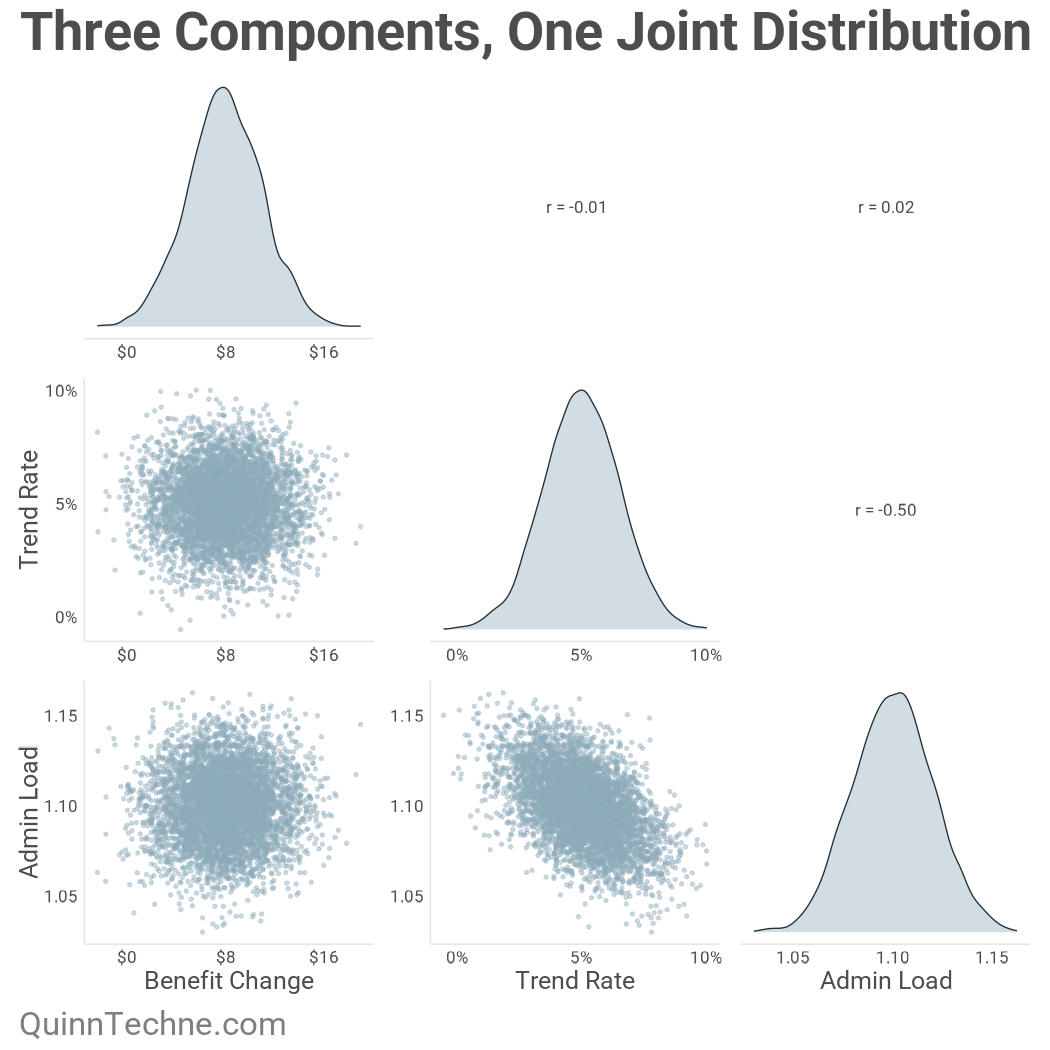

Here are the draws, unified under one distribution. These can then be aggregated into a cost distribution and compared to a selected rate to get a distribution of underwriting margin.

Up, Up, Down, Down, Left...

Tracking the full joint distribution might be beyond the skills or tools at hand. A first-order approximation of the underwriting margin distribution can be done by calculating and pushing through the means of all the subcomponents to create a rate and expected underwriting margin, then approximating the standard deviation of that distribution based on experience. Now actuaries could, in theory, track only one marginal distribution: The underwriting margin. (Don't try this at home! Keep track of more than one, please.)

$$E(\tilde{c} \mid y) \approx g(\mu_b, \mu_t, \mu_a)$$

\( \mu_b, \mu_t, \mu_a \): The component means, point estimates from each component model.
\( \approx \): "Approximately equals."

This equation estimates costs by inputting the mean of each component into our cost aggregating function. This is trading each rate component's full distribution for a summary statistic. You then have an underwriting gain distribution like this:

$$\tilde{u} \sim \text{N}\big(m, \; \text{sd}_{\text{exp}}^2\big)$$

\( \text{N} \): The normal distribution or bell curve, one variable this time.
\( \text{sd}_{\text{exp}} \): The margin spread directly dropped in (4% here). Generally, it's the block's historical realized-margin volatility.

This approximation has tradeoffs. One is Jensen's Inequality: the function evaluated at the means (this approximation) is not the mean of the function evaluated over the joint distribution. Convexity, like the trend application, and correlation open the gap. It's trivial in our example:

# Jensen gap: g() with means as inputs vs. the mean of g() using the joint distribution

# With means as inputs
cost_first_order <- (known_paid + mu_z["benefit_change"]) * (1 + mu_z["trend_rate"])^n_years * mu_z["admin_load"]

round(cost_first_order, 2)
[1] 494.8

# Mean of the cost function with the joint distribution as input
round(mean(cost), 2) 
# [1] 494.63

# Expected simulation noise: the Monte Carlo standard error of mean(cost)
mc_se <- sd(cost) / sqrt(n_draws)
round(mc_se, 2)
# [1] 0.18
  
# The gap (no, not that Gap)
round(cost_first_order - mean(cost), 2) 
# [1] 0.18 # Noise

Fortunately, the cost aggregation is fairly linear, minimizing any issue.

Other tradeoffs in this approximation:

• You cannot decompose how much each component contributes to the total spread. That said, aggregate standard deviations tend to be dominated by the largest-spread component, which is probably a trend component.
• You cannot intervene on a value and calculate a new distribution. This limits your "what if?" abilities.
• You are assuming the random variable's shape—likely that it's approximately normal.

What Could Go Wrong?

Recall, uncertainty is encoded in spread.

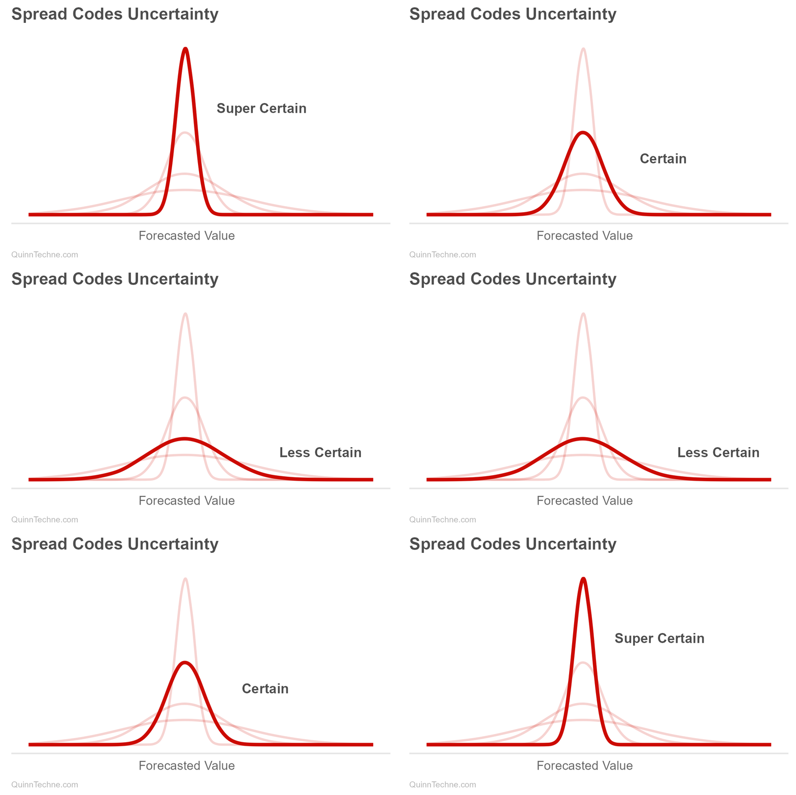
If the actuary incorrectly encodes uncertainty as conservatism, then the actuary's belief is lost. Do not bias your assumptions with conservatism. Similarly, the actuary may incorrectly try to encode uncertainty by selecting a scenario when they should have kept the entire distribution. For example, choosing the 90th percentile of trend and the 90th percentile of admin load as some adverse scenario and trying to combine the percentile values—which has problems, so don't do it. This math would produce a number, but it would be just that: a number devoid of probability. A quantitative scenario is only useful if it carries a probability. The principled path to recover one is to work out the joint probability distribution, push it through the cost function, and look at the cost distribution's cumulative distribution function at this chimeric value. Then you're back to having a probability.

The actuarial standards already warn against percentile stacking:

ASOP No. 56 — Modeling: 3.1.6.e. "Reasonable Model in the Aggregate—The actuary should assess the reasonability of the model output when determining whether the assumptions are reasonable in the aggregate."

It's not just conservatism that can be problematic, but focusing on isolated marginal distributions risks distracting from the joint probability distribution.

What’s an Actuary to Do?

1. Think in distributions. Keep them throughout your whole rate development as long as you can. Taking an average should be the last thing you're doing.
2. Don't bias your assumptions with conservatism.
3. Don't try to combine percentiles.
4. If you have a scenario or forecast but no associated probability: Stop, locate the nearest probability distribution—keeping in mind it may be behind you.

Actuarial Standards Board. (2010, December). ASOP No. 41: Actuarial Communications. Retrieved August 17, 2026, from https://www.actuarialstandardsboard.org/asops/actuarial-communications/

Actuarial Standards Board. (2019, December). ASOP No. 56: Modeling. Retrieved August 17, 2026, from https://www.actuarialstandardsboard.org/asops/modeling-3/

Gelman, A., Carlin, J. B., Stern, H. S., Dunson, D. B., Vehtari, A., & Rubin, D. B. (2013). Bayesian Data Analysis (3rd ed.). CRC Press.

Calculations and graphics done in R version 4.3.3.

Qiu Y (2024). showtext: Using Fonts More Easily in R Graphs. R package version 0.9-7. https://CRAN.R-project.org/package=showtext

Pedersen T (2024). patchwork: The Composer of Plots. R package version 1.2.0. https://CRAN.R-project.org/package=patchwork

Venables WN, Ripley BD (2002). Modern Applied Statistics with S (MASS), Fourth edition. Springer, New York. https://www.stats.ox.ac.uk/pub/MASS4/

Wickham H, et al. (2019). Welcome to the tidyverse. Journal of Open Source Software, 4 (43), 1686. https://doi.org/10.21105/joss.01686

The views and opinions expressed in this article are those of the author and do not represent the official policy or position of any employer, organization, or entity. This article is for informational and educational purposes only and does not constitute professional actuarial advice.

Generative AIs like Anthropic's Claude Fable 5 were used in parts of the writing review and coding. The author did the Suminagashi cover.