Mirror, Mirror, on the wall, who is the most likely of them all?
We build models to understand the world and plan accordingly. Our beliefs about the world, including forecasts, are distribution-shaped: we believe some values, or hypotheses, are more plausible than others. Write out those hypotheses and how plausible you think they are; that's a distribution. When charted, the taller parts of the distribution are where the more plausible values are on your horizontal x-axis. Distributions encode the plausibility of outcomes, or, call it, probabilities. All probability is conditional—we know things about the world. Thus our distributions are also conditional. Moreover, we can update our distributions with new data. How much we update depends on two things:
- How certain we are in our prior belief
- The strength of evidence from the new data, qualitative or quantitative
Behold, Bayes' theorem.
$$p(\theta \mid x) = \frac{p(x \mid \theta) p(\theta)}{p(x)}$$
\(p(·)\): Plausibility of the thing.
\(θ\) (pronounced theta): It can be a number, several numbers, a category, or even a whole distribution, as long as it says what data to expect.
\(x\): The observed data.
\(|\): “Given”; everything to its right is treated as known.
\(p(θ)\): The prior, or your belief based on background information and before seeing \(x\), the data.
\(p(x | θ)\): The likelihood, how well each value of \(θ\) predicts the data.
\(p(θ | x)\): The posterior, your prior updated as your new belief after seeing the data.
\(p(x)\): The likelihood averaged over all values of \(θ\), weighted by the prior.
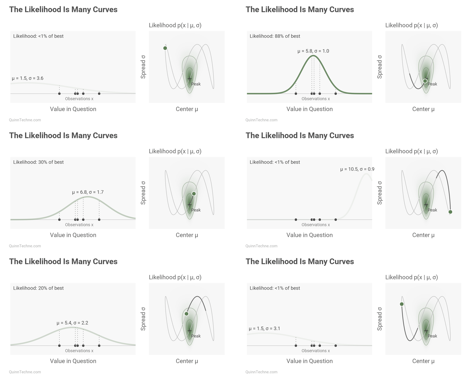
Sometimes the data source is questionable. Sometimes we face multiple reasonable sources that don’t agree. Sometimes the new information is qualitative, or information that makes us reinterpret past data. Formally, the likelihood function encodes how each given value of \(θ\) predicts the new information. \(x\) best in \(p(x | θ)\)? Which is then a step in learning what \(θ\) to update towards in \(p(θ | x)\), our posterior. The likelihood is not a single value. It is a function—a shapeshifter. You can evaluate how probable \(x\) is given input values of \(θ\). You have to assume the shape of the data (Normal, Poisson, Binomial, etc.). That choice, and other features, is how we'll see the likelihood encode our trust in the data source. First, here's an example of sweeping over various Normal curves and how some combinations of \(θ\) (our mean and standard deviation parameters) predict the data better than others. The better prediction is where the animation slows down and the line becomes darker.
It's also up to you to assess whether the data matches the same basis as your prior—that the data is relevant: measured the same way, sampled the same way, that it depends on \(θ\) at all. Imagine you were trying to forecast future insurance losses related to apple crops in Washington. Let’s call our \(\theta\) the distribution of next year's aggregate losses. Then you get data on elephant birth weights in Indonesia during full moons. What is your likelihood function? The two are unrelated. Any value we’re worried about has no bearing on the birth weights. Imagine you have a crop-insurance-elephant-birth-weight function, and no matter how you change your insurance assumptions, you always get back the answer “who cares?!” It’s a flat line because the value is the same everywhere. The birth-weight answer is the same for every apple-crop \(\theta\) used. It carries no information. Our posterior remains at the prior because we have learned nothing to update on. Ideally, we prevent unrelated data from even entering the model. However, the idea of flatness and a posterior that moves little from its prior is still a useful concept.
Who Did You Say You Were?
When we get data, we may be unsure how trustworthy the source is. We can blend how much we update the model with the data versus taking it at face value. See the example of what I call the learning rate:
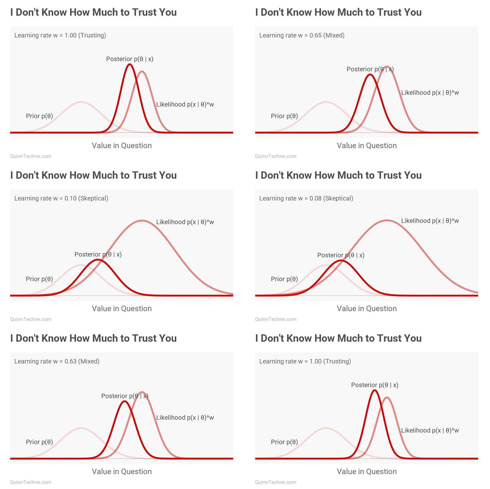
As seen above, in a strong-evidence case, the likelihood is concentrated and spiked, or taller, on a smaller range of values. Uncertainty, by contrast, flattens the likelihood toward a line; we’re unsure of anything the source says, even if it falls near our prior! If the data source is questionable, give it a wider likelihood and update less than you otherwise would. If the source is known to be consistent, give it a narrower, more certain likelihood, and update more. I say consistent because we have been discussing what it means not to know whether to trust. This is different from knowing a source is consistently untrustworthy. We'll talk later about when a source is consistently untrustworthy. That case is also a different likelihood function than if you know the source is trustworthy but sometimes gives errors.
My Bad
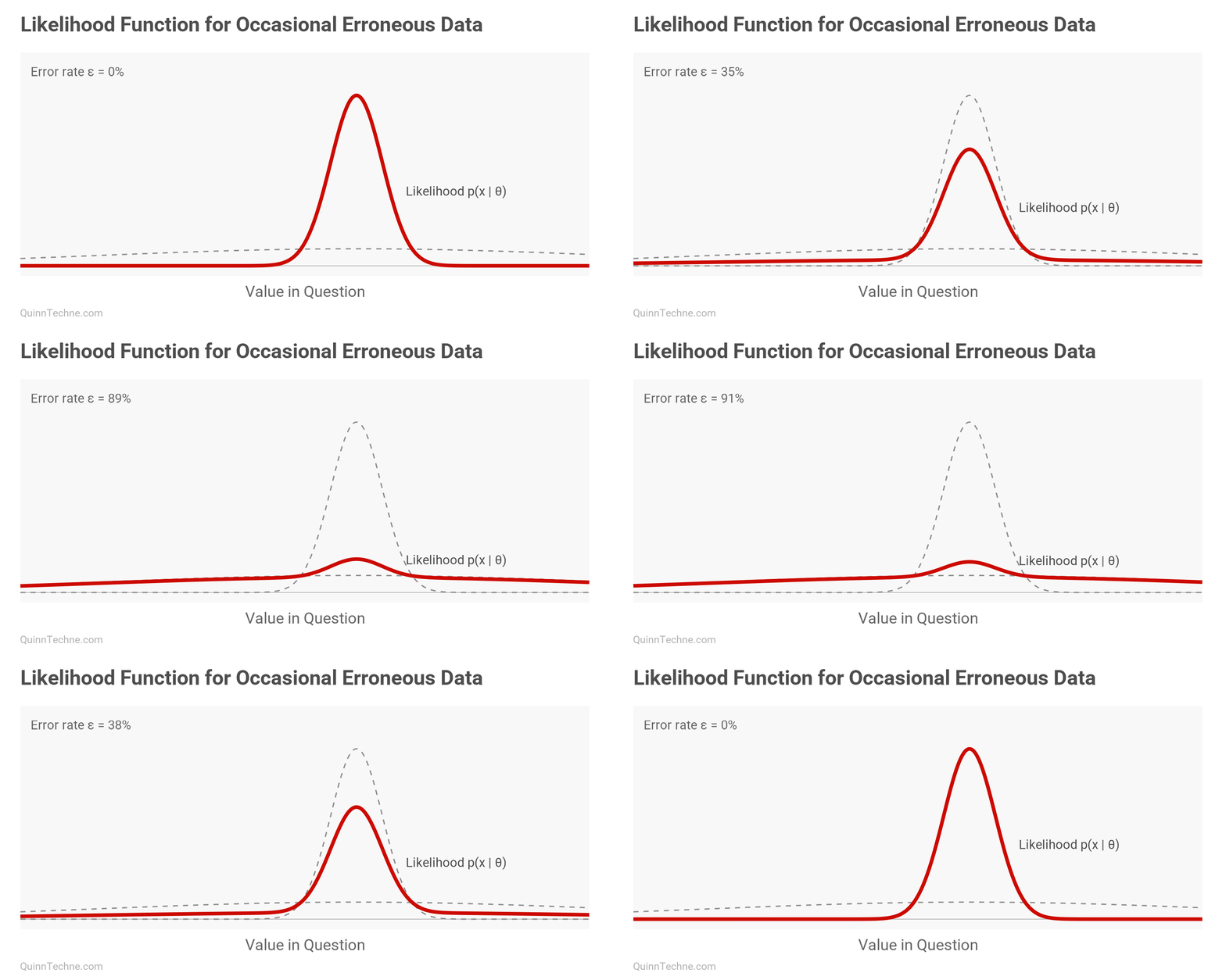
Suppose a source sometimes reports erroneous data. Start with the distribution you would use if the source were always accurate, then blend this chosen function with a flat line. The flat line absorbs outlier values that would otherwise pull the posterior toward them. Besides flat lines, you might also see a Student's t-distribution with wider tails, or a mix of a narrow and a wide Normal distribution as shown next:
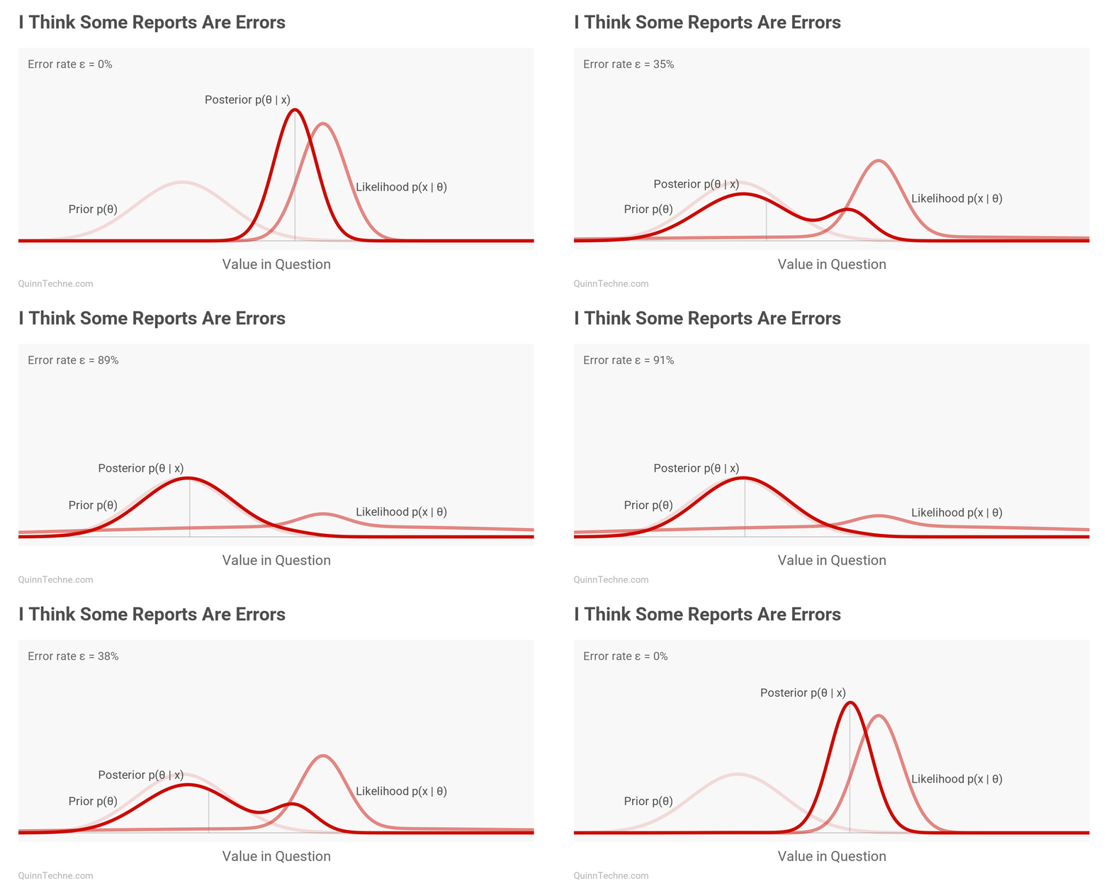
Agree to Disagree
Actuarial Standard of Practice (ASOP) No. 1 explains how two actuaries, faced with the same facts, may reach different conclusions. This is valid from a Bayesian viewpoint because the actuaries may see the same evidence and assign the same likelihood but start with different priors. The actuaries might be closer to agreeing than before, but not fully. If their posteriors noticeably overlap, this is closer to agreeing than little to no overlap. When there's overlap, then they're probably pointing at the same phenomenon even if they report different point estimates. (You're wrong because I say 5.4%, and you said 5.3%! Oh, if only they had distributions to share.)
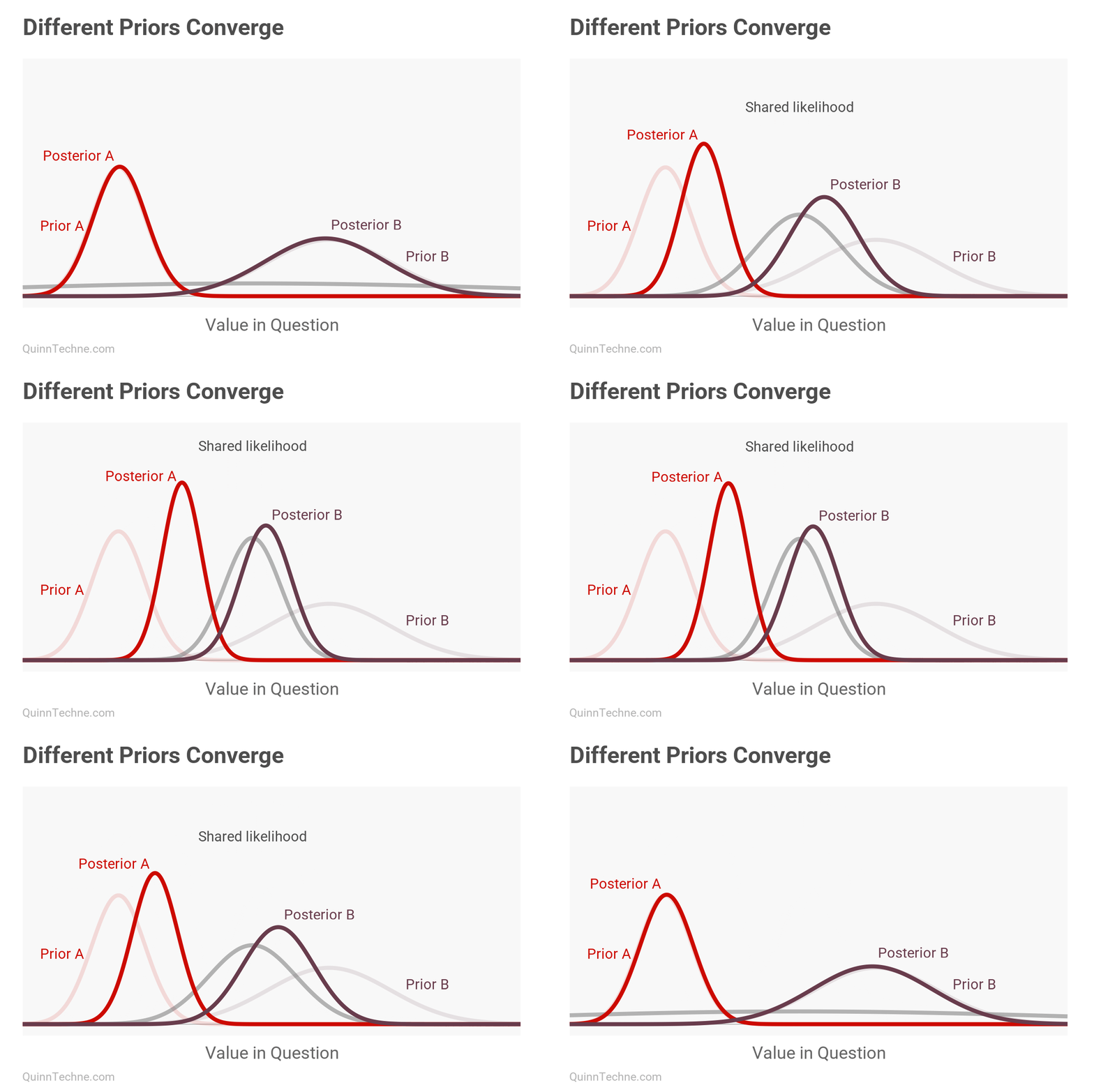
Usually, reality is more complicated. The same data may elicit different likelihoods from each actuary. One actuary might trust the data source while the other is more skeptical: different likelihood functions, different posteriors—all from the same data.
Distrust as a Signal
Sometimes different likelihoods lead to divergent opinions after two people see the same data. Consider this quote from The Economist: “Yet Russians, hardened by experience, tend to think that the more emphatically authorities deny planning something unpleasant, the more likely it is to happen.” In the next chart, suppose person [A] trusts the government source and person [B] does not. Denying is a signal. They start at the same prior but end with opposite conclusions after seeing the same data. This is due to their likelihood functions. Person [B] thinks authorities deny more when they are planning something unpleasant, so [B] thinks \(p(\text{deny} | \text{unpleasant})\) is larger than \(p(\text{deny} |\text{pleasant})\), that denying happened more in the world where unpleasant things happened.
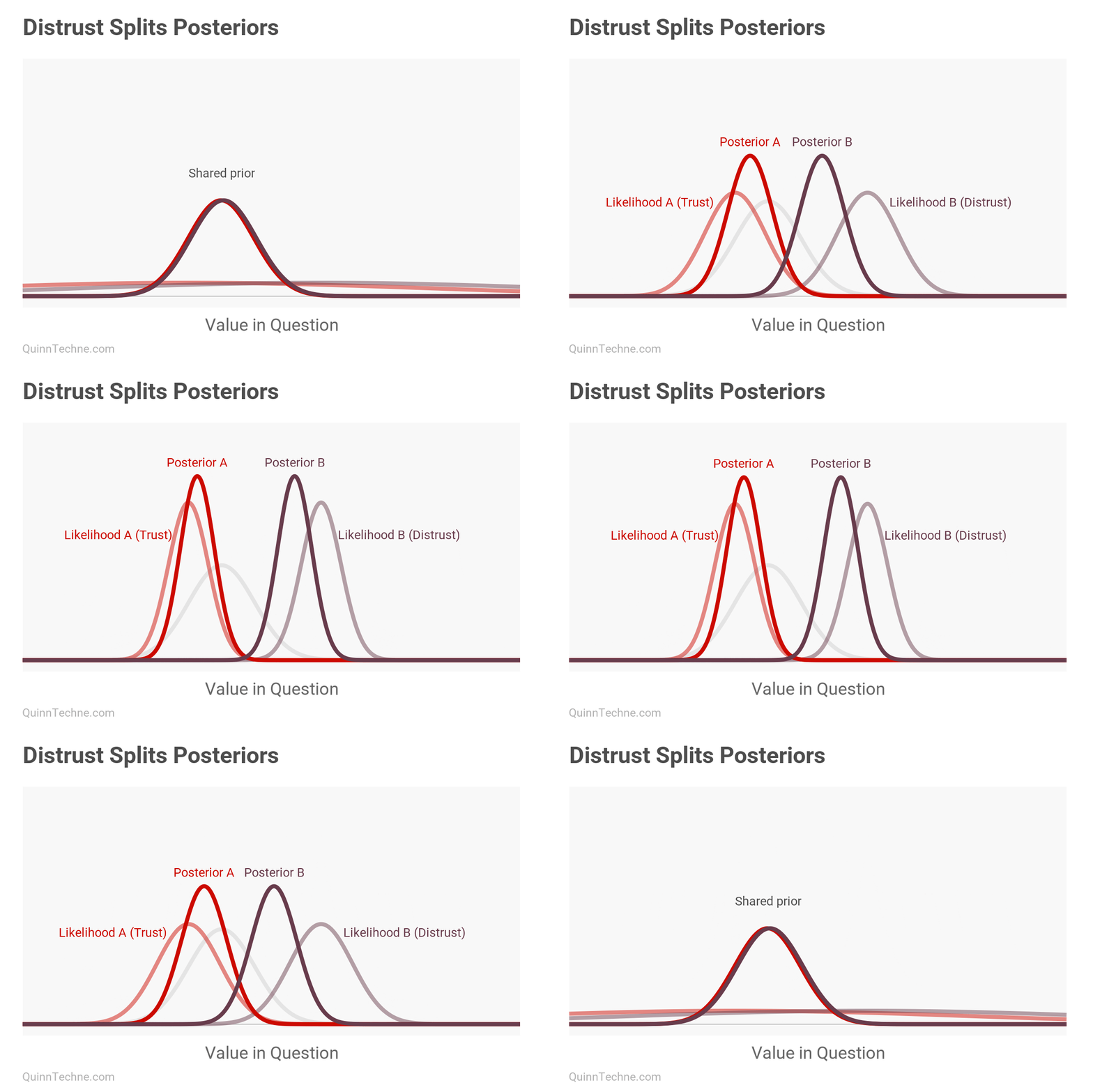
I want to highlight that active distrust is different from uncertainty. The very first examples were about unknown sources, and the likelihoods flattened. Distrust is a mirroring of trust—you still get a signal from a distrusted source. You just need the source to be consistent.
Mirror, Mirror
When building statistical models for forecasting, I sometimes hear others accuse me of "trusting the data too much." No. That type of trust can be accommodated in the modeling. It's the actuary not being explicit about their likelihood function that we might distrust.
Actuarial Standards Board. (2013). Actuarial Standard of Practice No. 1: Introductory Actuarial Standard of Practice. http://www.actuarialstandardsboard.org/asops/introductoryactuarialstandardpractice/
Bissiri, P. G., Holmes, C. C., & Walker, S. G. (2016). A general framework for updating belief distributions. Journal of the Royal Statistical Society: Series B (Statistical Methodology), 78(5), 1103–1130. https://doi.org/10.1111/rssb.12158
Calculations and graphics done in R version 4.3.3, with these packages:
Wickham H, et al. (2019). Welcome to the tidyverse. Journal of Open Source Software, 4 (43), 1686. https://doi.org/10.21105/joss.01686
Pedersen T (2024). patchwork: The Composer of Plots. R package version 1.2.0. https://CRAN.R-project.org/package=patchwork
Qiu Y (2024). showtext: Using Fonts More Easily in R Graphs. R package version 0.9-7. https://CRAN.R-project.org/package=showtext
Ooms J, Lesiński K (2025). gifski: Highest Quality GIF Encoder. R package version 1.32.0-2. https://CRAN.R-project.org/package=gifski
Generative AIs like Anthropic's Claude Opus 5.5 were used in parts of coding and reviewing the writing. The Suminagashi cover was done by the author.